Bluecoat Proxy Big Analysis

This article is a step-by-step tutorial aiming at loading and analyzing the bluecoat_proxy_big.zip dataset from Public Security Log Sharing in Squey.
The first section is devoted the creation of a parsing file that will allow us to load the dataset. Should you be in a hurry, you can skip straight to the analysis as the file is provided below.
Parsing file creation
Before being able to load the dataset into the application, a parsing file (called format) should be created using the Format Builder tool.
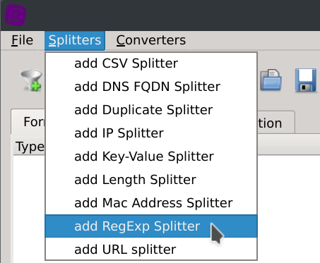
Click on the Create a new format... button located on the start page and then on the Splitters > add RegExp Splitter menus.

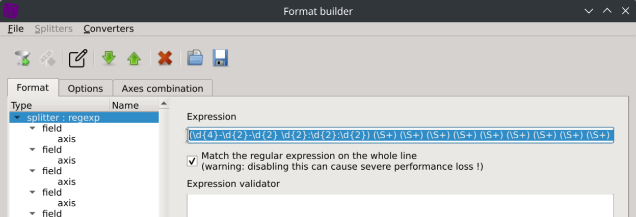
Enter the following regular expression into the Expression text field:
(\d{4}-\d{2}-\d{2} \d{2}:\d{2}:\d{2}) (\S+) (\S+) (\S+) (\S+) (\S+) (\S+) (\S+) (\S+) (\S+) (\S+) (\S+) (\S+) (\S+) (\S+) (\S+) "?(-|[^"]*)"? (\S+) (\S+) "?(-|[^"]*)"? (\S+) (\S+)[ ]?"?(-|[^"]*)"?[ ]?(\S+)?[ ]?"?(-|[^"]*)?"?
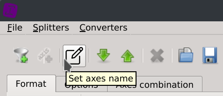
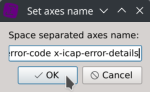
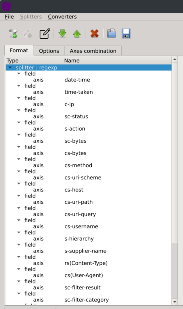
Then click on the Set axes name toolbar button and copy/paste the following columns name in the text dialog:
date-time time-taken c-ip sc-status s-action sc-bytes cs-bytes cs-method cs-uri-scheme cs-host cs-uri-path cs-uri-query cs-username s-hierarchy s-supplier-name rs(Content-Type) cs(User-Agent) sc-filter-result sc-filter-category x-virus-id s-ip s-sitename x-virus-details x-icap-error-code x-icap-error-details
Note: thoses were extracted from the log file using the following command:
sed -n '4p' Demo_log_001.log | cut -d" " -f2- | sed 's/ /-/'
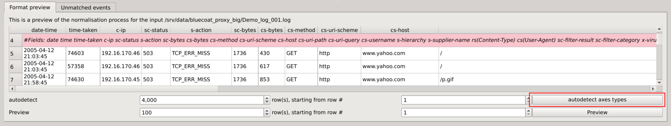
Loading a file of the dataset will now help you confirm that the data is appropriately parsed but will also automatically detect the types of the columns.
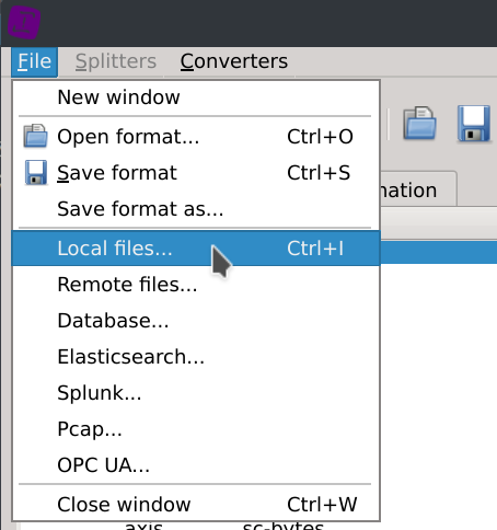
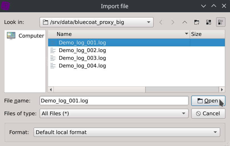
Click on the File > Local files... menus and select one of the dataset log file.
Click on the autodetect axes types located in the bottom right corner of the dialog.
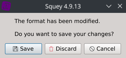
Finally, save the format as squey.format in the bluecoat_proxy_big directory
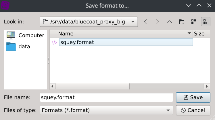
Note that squey.format is a catch-all name that will automatically match any dataset, and that’s handy for datasets composed of several files. To match a specific dataset, say dataset.csv, name your format dataset.csv.format. If your format name doesn’t match a dataset name, you will have to explicitely select it at loading by selecting Format: custom format and a dialog box will ask you to locate it on the disk.
Loading the dataset
If not done previously:
- Download and extract the dataset on your machine.
- Download and and extract squey.format.zip in the same folder the dataset was extracted.
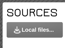
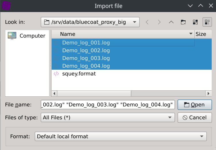
Click on the Local files... button located on the SOURCES section of the start page and select the dataset log files.
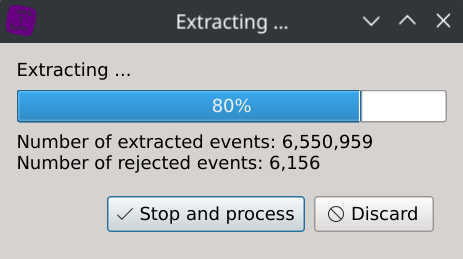
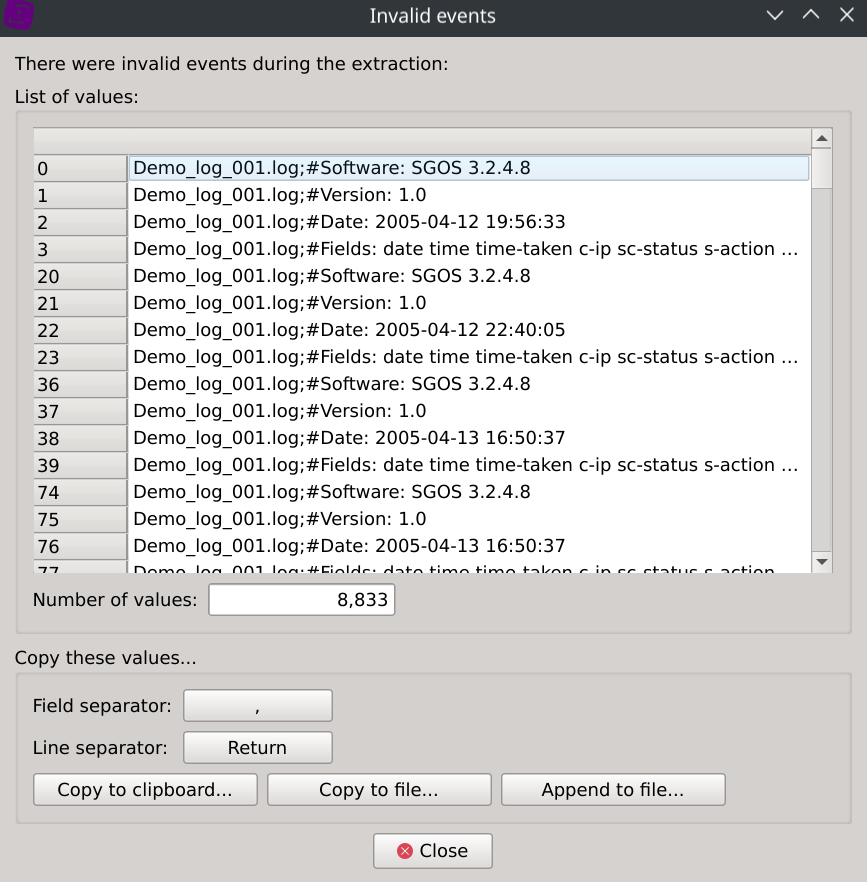
During the data ingest stage, it was found that 8,883 rows (~0,11%) were dismissed.
A dialog is displaying them so you can confirm after inspection that they are all redundant headers and no other valuable data was left out.
It took 16.22 seconds to load the dataset (4 text files, ~2.6GB uncompressed data) on an Intel® Core™ i7-12700H Processor and the memory consumption was ~5GB.
It took only 2.96 seconds to reload the saved investigation from disk (~1.1G binary data) as the data ingest stage alredy occured.
Note that in case your dataset is exceeding the available memory of your system, you can always filter out some rows during the data ingest stage by applying custom exclusion rules to specific columns and make your analysis in several steps.
Visual analysis
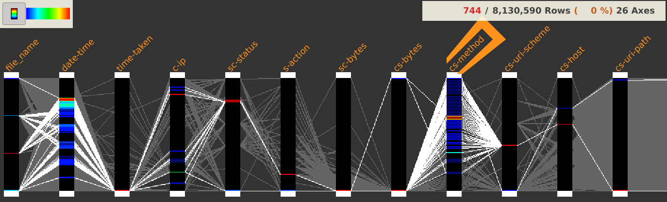
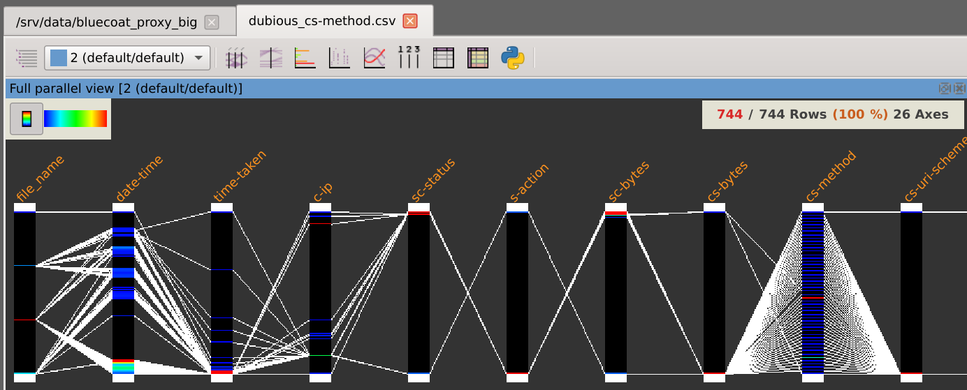
After loading the dataset, it is displayed in integrality using parallel coordinates.
To gain more knowledge about how the parallel coordinates work in Squey, please ensure to have read the according section of the documentation.
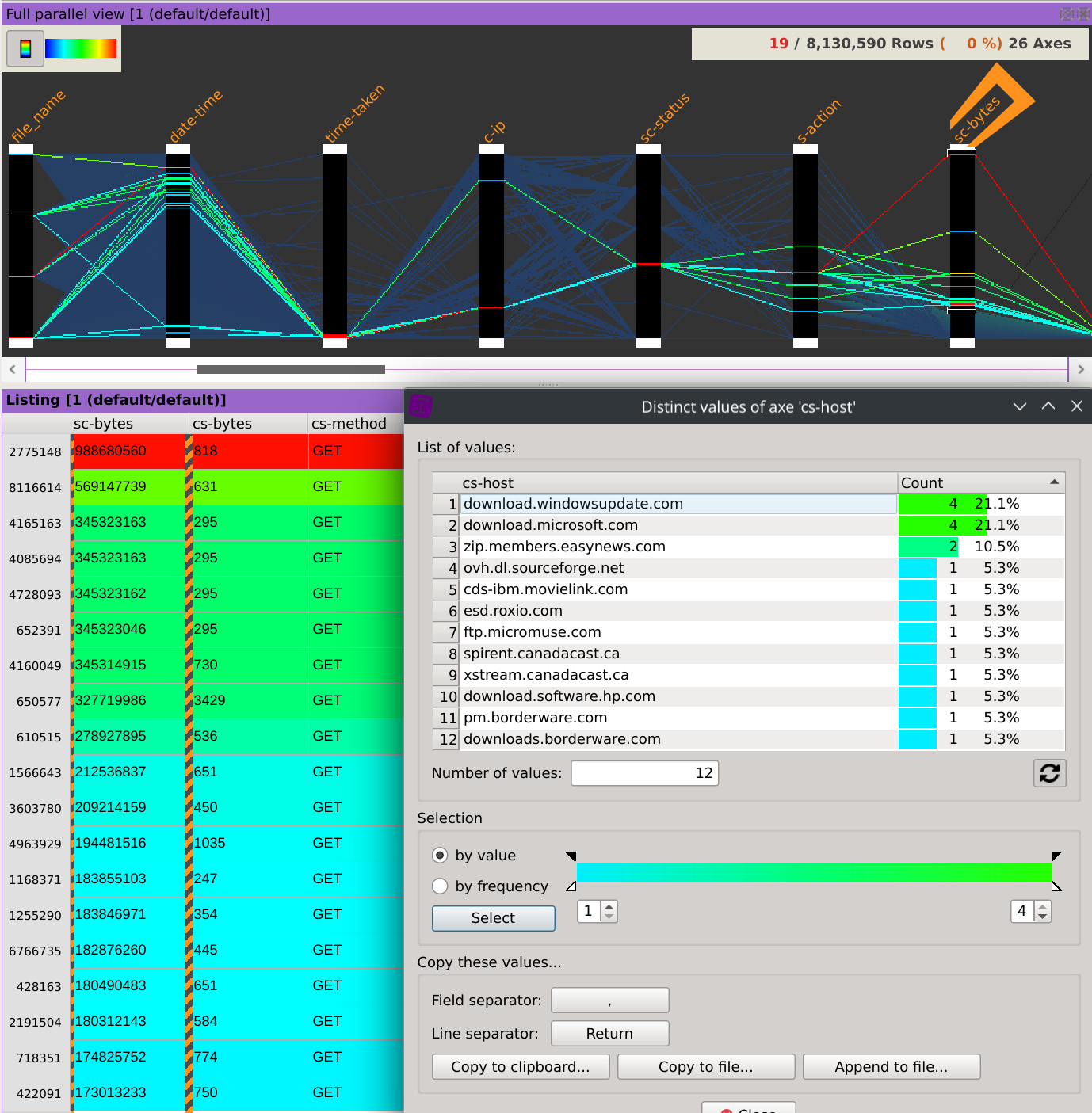
This dataset is composed of 8,130,590 rows and 26 columns and looks like this:
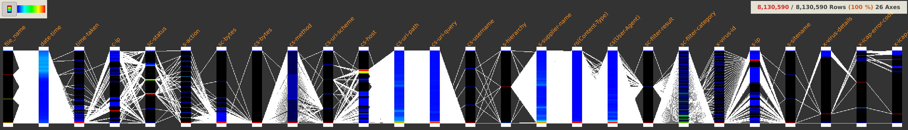
A first look at the displayed axes could already make us discover some facts worth of interest.
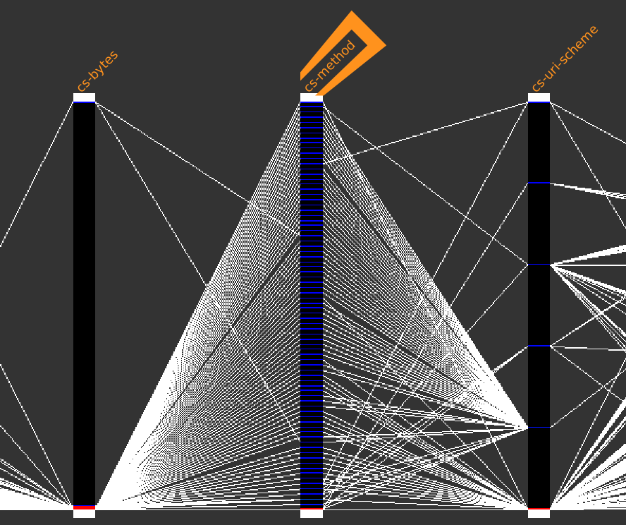
Dubious cs-method
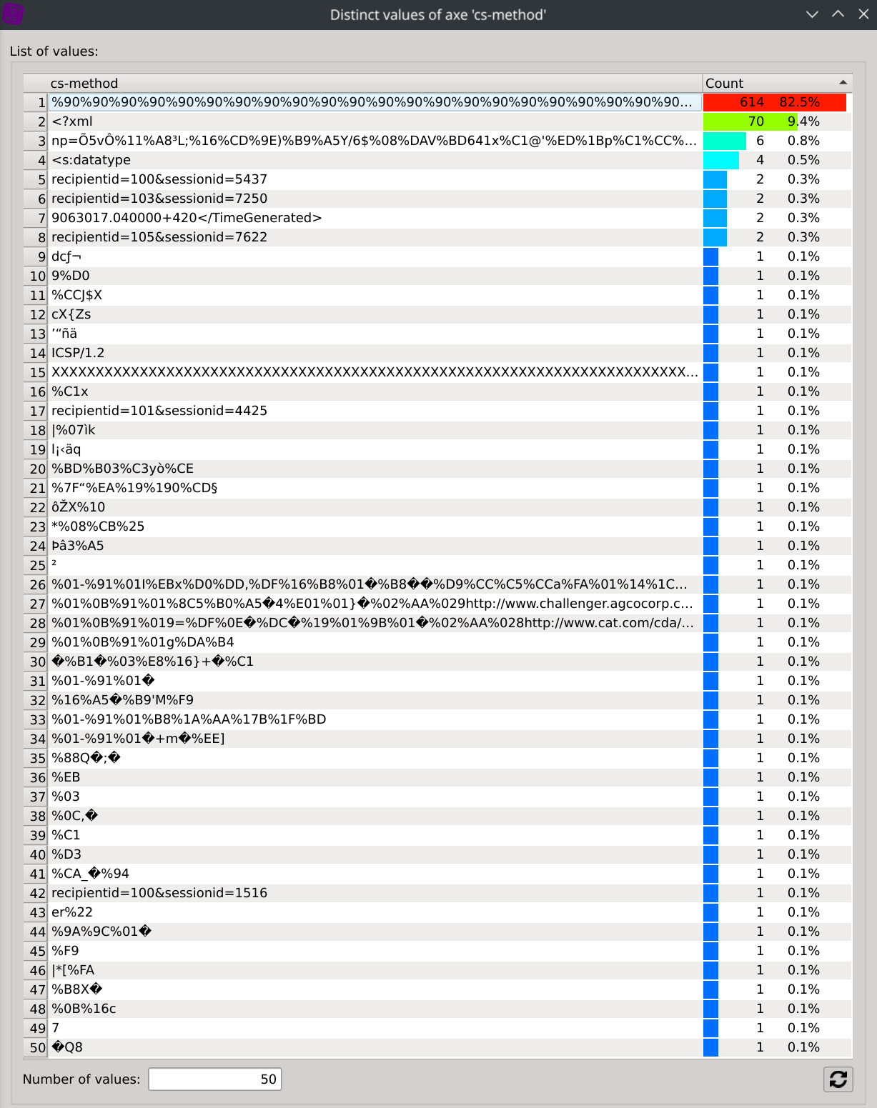
Anyone a bit familiar with proxies would probably ask himself why the cs-method column is containing so much different values ?
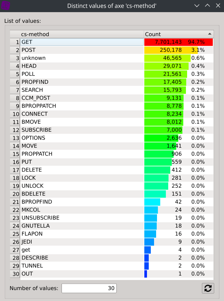
A right-click on the cs-method column header and selecting Distinct values display each distinct values as well as their associated count.
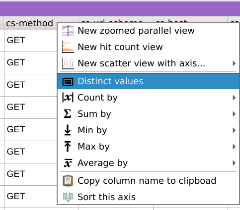
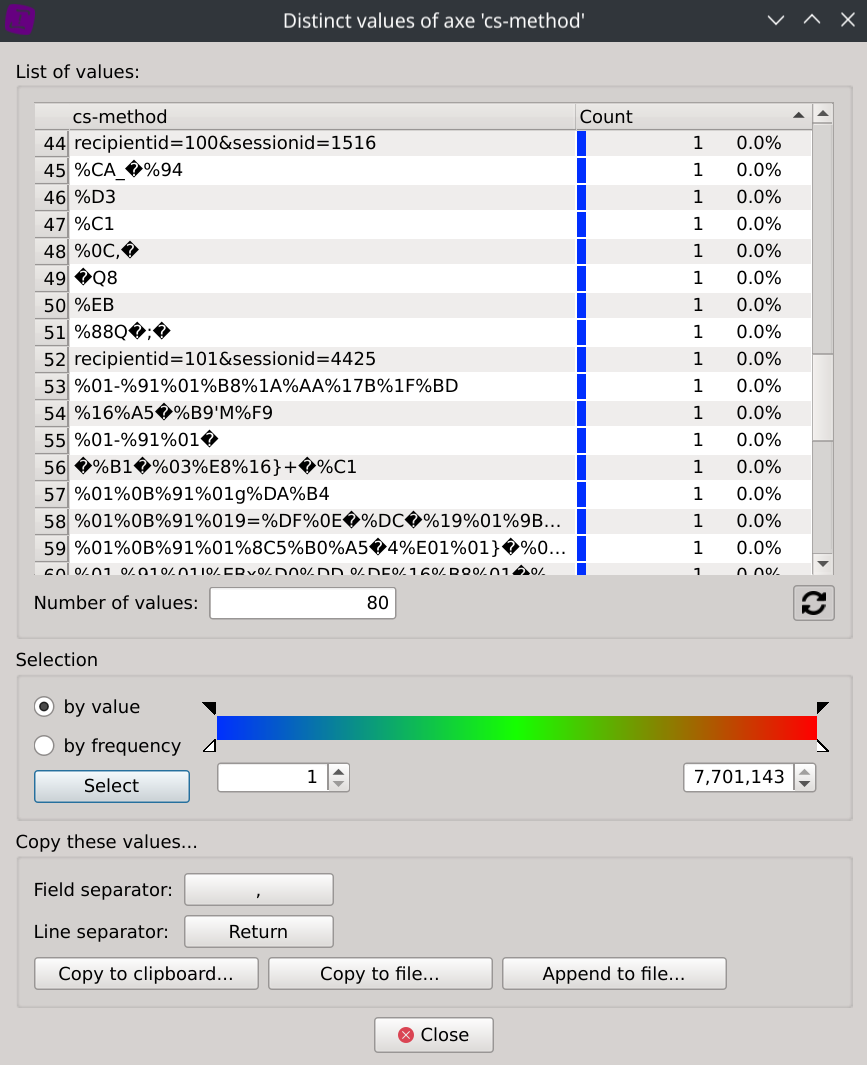
We can then observe that many of them do not look to methods of standardized protocols but seem rather unusual.
Before going any further, let’s clear our mind from any doubt that this could come from a corruption during the data download or ingest stage.
Here are the SHA-256 checkums of the files composing the dataset:
[/srv/data/bluecoat_proxy_big]$ sha256sum *
db1b8371cbee4a6ff3755c11d5aad81aab4661449b0c5eac14f2f93b9b0b0bf9  Demo_log_001.log
8ff4858536215473e752db29537e46f598e79dd9985f15eedda85115d3c4fd0f  Demo_log_002.log
18759422a0836e61ddc1f2877ba7ae516179f07675a39e2fa8d9bf6baa238731  Demo_log_003.log
27139f8d611686127733e2a0eaf67eaf12e616332bc2cc281ec50af4984518b3  Demo_log_004.log
And here are some of the rows extracted from the original data:
sed -n '981185p; 1070757p; 1151521p; 1168033p; 1252127p; 1516636p; 1570191p; 1613877p; 1817343p; 1843350p; 1844162p; 1844203p; 1844351p; 1847392p; 1847641p; 1847644p; 1861554p; 2185718p; 2561934p; 2648396p; 2747923p; 2962884p; 2962885p; 2963953p; 3019317p; 3023657p; 3164071p; 3165808p; 3172156p; 3329713p; 3382352p; 3591245p; 3709973p; 3741054p; 3743310p; 3745850p' Demo_log_003.log
2005-05-03 16:36:32 3598 45.112.1.58 400 TCP_NC_MISS 9036 4294967282 %03 - - / - - NONE 192.16.170.44 - - PROXIED unavailable - 192.16.170.44 SG-HTTP-Service - - -
2005-05-03 17:30:50 10031 45.116.1.30 0 TCP_ERR_MISS 0 12 7 - - / - - NONE - - - PROXIED none - 192.16.170.44 SG-HTTP-Service - - -
2005-05-03 18:07:26 1 45.116.1.30 400 TCP_NC_MISS 9036 12 %0B%16c - - / - - NONE 192.16.170.44 - - PROXIED unavailable - 192.16.170.44 SG-HTTP-Service - - -
2005-05-03 18:16:30 1 45.116.1.30 400 TCP_NC_MISS 9036 12 %B8X� - - / - - NONE 192.16.170.44 - - PROXIED unavailable - 192.16.170.44 SG-HTTP-Service - - -
2005-05-03 19:01:13 1922 45.14.2.150 0 TCP_ERR_MISS 0 16 |*[%FA - - / - - NONE - - - PROXIED none - 192.16.170.44 SG-HTTP-Service - - -
2005-05-03 21:33:05 459 45.14.3.123 0 TCP_ERR_MISS 0 16 %F9 - - / - - NONE - - - PROXIED none - 192.16.170.44 SG-HTTP-Service - - -
2005-05-03 22:02:36 485 45.114.2.68 0 TCP_ERR_MISS 0 16 %9A%9C%01� - - / - - NONE - - - PROXIED none - 192.16.170.44 SG-HTTP-Service - - -
2005-05-04 00:08:09 1 45.21.4.254 400 TCP_NC_MISS 9036 34 recipientid=100&sessionid=1516 - - / - - NONE 192.16.170.44 - - PROXIED unavailable - 192.16.170.44 SG-HTTP-Service - - -
2005-05-04 00:35:42 9 45.114.3.11 400 TCP_NC_MISS 9036 679 <?xml - - / - - NONE 192.16.170.44 - - PROXIED unavailable - 192.16.170.44 SG-HTTP-Service - - -
As we can see, these were well present in the original data.
This leaves us with at leat two hypotheses.
First, this could be a bug in the proxy OS that could arise under heavy load. In that case, it could be useful to take some mitigation measures like upgrading the sofware, monitoring the CPU usage, reducing the bandwidth usage, redesigning some part of the network or upgrading the hardware.
Secondly, this could be bogus communications of faulty apps that could be reported upstream, or malicious communications that should be further investigated.
Exporting our first discovery
Let’s export this isolated data subset for a potential investigation before focusing on our main analysis.
There is two ways to isolate these dubious cs-method values:
- Select any wanted values from the
Distinct valuesdialog - Filter out valid values by applying a search regular expression
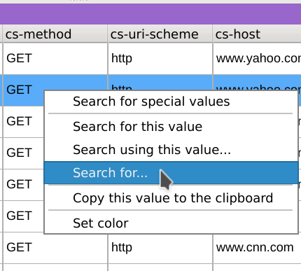
Let’s try the second approach: right-click on any values of the listing in the cs-method column, select Search for..., copy the following regular expression [A-Za-z_]*, select exclude and Regular expressions and click apply:
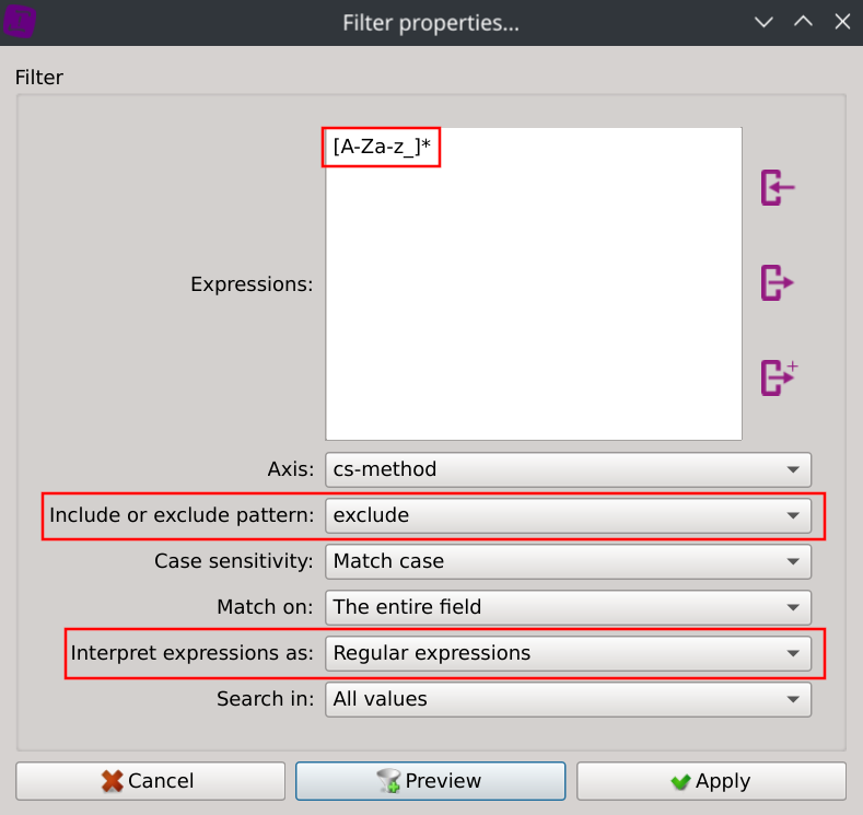
This instantly filtered our dataset:
Displaying the distinct values of the cs-method column now only shows the selected values:
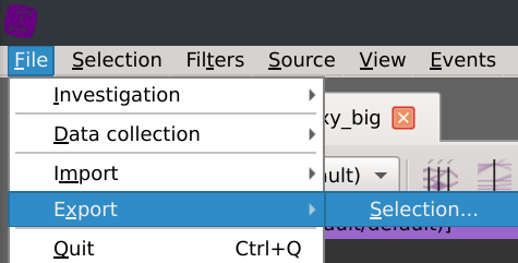
We can then export the selected rows by clicking on the File > Export > Selection menus.
On-the-fly compression is supported with the following formats: gz, bz2, zip and xz.
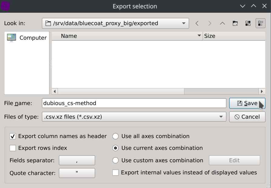
The dataset has been exported to dubious_cs-method.csv.xz (5.1KB).
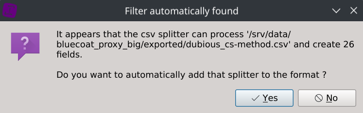
It can easily be loaded back into the application with on-the-fly decompression, headers and columns type autodetection.

Creating our first layer
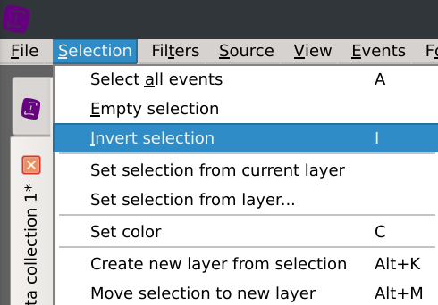
Note that inverting the selected rows can be done by clicking on the Selection menu and selecting Invert selection (I).
The Distinct values dialog is then automatically updated to display the trusful cs-method values and their associated count/percentage:
This should give us a better understanding of the different protocols at work.
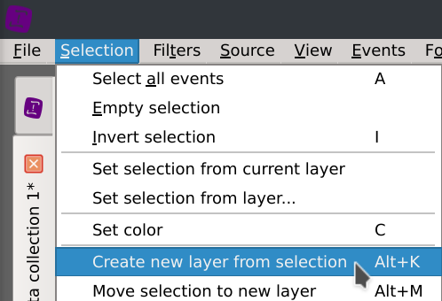
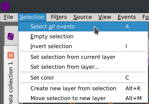
To confortably continue our analysis, let’s isolate the current selected rows in an active layer so that these dubious cs-method values won’t stood in the way anymore. Click on the Selection > Create new layer from selection (Alt+K) menus and give your layer the name you want.
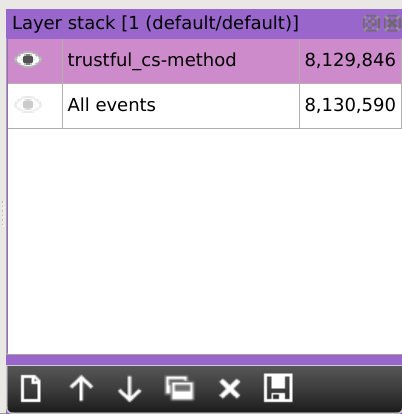
As you can see on the layer stack, our active dataset is now restricted to the rows with trustful cs-method values: we let aside 744 identified rows.
Back to our main analysis
Should there be a bandwidth problem, let’s try to understand how it is distributed across the traffic.
Note: coloring the rows using a gradient of color depending on the size of the requests can opionally be done by clicking on Filters > Axis gradient menus and selecting the sc-bytes axis.
Right-click on the sc-bytes axis title, select New selection cursor and select the top of the axis to filter high values.
We can see which requests are consuming a lot of bandwidth as well as their associated hosts. This is interesting but we are still missing the big picture as lots of contents are not fetch in a single request but with many of them.
It would be nice if we could aggregate values of a selected column by doing a sum on numeric values located on another column.
Fortunately we can do this easily using the Sumby function.
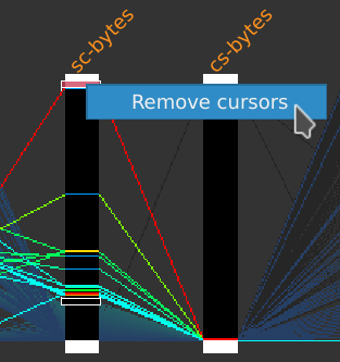
First, remove the selection cursors by right-clicking on one of them and select Remove cursors, then click on the Selection > Select all events menus.
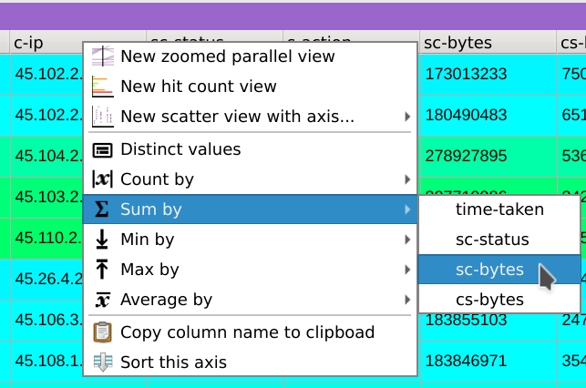
Finally, right-click on the header of the c-ip column, select Sum by and then click on the sc-bytes column.
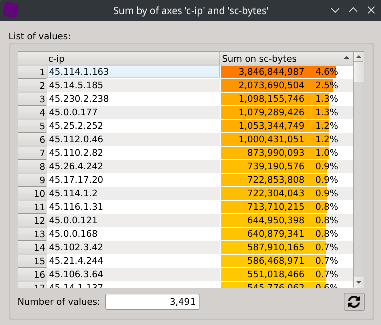
This displays the distinct values contained in the c-ip column, but instead of displaying a count based on the frequency of which they appears, the dialog now displays their consumed bandwidth.
To gain even more information about the supposed types of traffic of each IPs, we can display the consumed bandwidth of each hosts. Right-click on the header of the cs-host column, select Sum by and then click on the sc-bytes column.
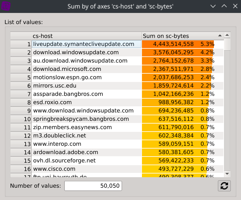
What could really came in handy is that selecting a specific IP will instantly filter the dataset and refresh the second dialog, revealing the bandwidth repartition by hosts for this IP.
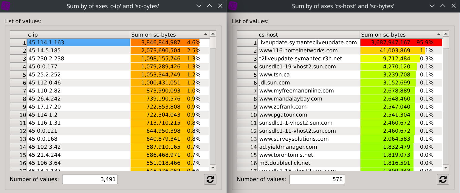
In this case, we can for example observe than IP 45.114.1.163 has downloaded ~3.43GB from liveupdate.symantecliveupdate.com, which represents 95.9% of its total traffic.
Continue the exploration on your own
Now that you master the basic features of Squey, feel free to continue exploring this dataset to discover additional insights.